EVo Model Description
EVo is designed to model the isothermal ascent of magma during eruption, assuming that magma degassing during ascent is primarily due to the resultant pressure change. A 3-phase system is used, where the silicate melt and the gas phase coexist in constant thermochemical equilibrium, alongside a solid graphite phase under sufficiently reduced conditions. The physical-chemical separation of gas and melt is implemented as being either impossible (closed-system), or instantaneous (open system - see Run types, set-up options and input parameters). The highly complex nature of volcanic systems necessitates simplifications in my approach; crystallisation kinetics and sulfide formation (see Handling additional phases: carbon and sulfur) are neglected, so in those cases where precipitation of solids during ascent is important in driving degassing, EVo may underestimate the volume and composition of gases evolved from the melt.
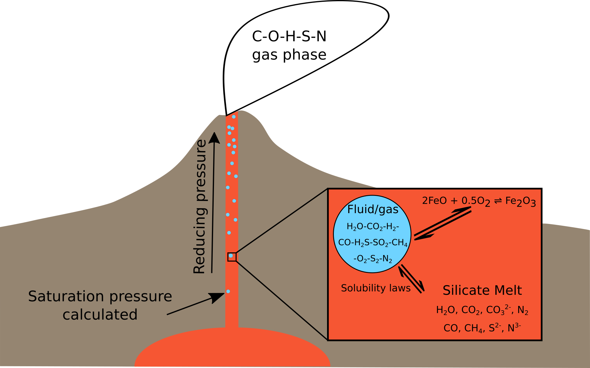
Fig. 1 A schematic overview of EVo, and it’s place in a physical system.
Fig. 1 shows a schematic of how EVo represents a volcanic system, calculating the composition of the gas and melt phase at stages from the pressure of volatile saturation to the surface.
Overview of the chemical model
EVo computes the gas and melt volatile composition for systems of up to 5 volatile elements (C, O, H, S and N, in combinations of OH, COH, SOH, COHS and COHSN), using an ‘equilibrium constants and mass balance’ method first established by Holloway (1987) and used since by several degassing models, including Iacono-Marziano et al. (2012), Gaillard and Scaillet (2014), and Burgisser et al. (2015). As stated by Holloway (1987), this method “requires that enough equilibrium constant equations are used so that, when combined with the equation for mass balance, there are an equal number of equations and unknowns”. By combining the equilibrium constant equations which define homogenous gas-gas equilibria, and solubility laws which control heterogeneous gas-melt equilibria, at any given point the entire gas-melt system can be defined.
EVo considers 10 gas-phase species in the full COHSN system: H2O, H2, O2, CO2, CO, CH4, S2, SO2, H2S and N2. Subsets of these species are used in calculations if systems with fewer components are modelled, e.g., by definition the COH system does not include S or N-bearing species and so comprises just 6 gas-phase species. In a typical terrestrial volcanic gas, \(>\)99% (by mol) will be made up of H2O, H2, CO2, SO2, H2S and N2 (Fischer and Chiodini, 2015), so the 10 species EVo considers are sufficient to model the bulk gas-phase chemistry, although it omits some trace species such as which have been detected at various volcanoes (e.g., Mori and Notsu, 1997; Oppenheimer and Kyle, 2008; Sawyer et al., 2008). OCS in particular has been omitted due to the lack of solubility data in magmas. This reflects a limitation of this approach: even when the homogenous gas-phase equilibria are known (which for very many species they are), unless there is corresponding data for the solubility of a species in silicate liquids it cannot be included and a self-consistent solution be obtained.
A set of five homogenous gas-phase equilibria, described in (1) to (5), define the speciation of the gas phase
At thermochemical equilibrium, the abundance of each species in the gas phase are related to an equilibrium constant, \(K_i\), one for each reaction in (1) to (5). The general equation for these equilibria is given by
which has a general equilibrium constant reaction equation of
where square brackets denote activity. For real gases, \(K_i\) can be calculated in terms of fugacity, \(f_i\), so that for, e.g., Eq. (1)
The fugacity \(f_i\) of a real gas is an effective partial pressure, which replaces the mechanical partial pressure in an accurate computation of the chemical equilibrium constant. In EVo ideal mixing of real gases is assumed, so the fugacity of species \(i\) is defined as
where \(\gamma_i\) is the fugacity coefficient representing the deviation of the gas from ideality, so for an ideal gas \(\gamma_i\) = 1. \(P_i\) is the partial pressure of \(i\), \(x^v_i\) is the mole fraction of i in the gas mixture, and \(P\) is the total pressure. \(x^v_i\) is such that when the gas phase is composed of \(n\) species, each with a mole fraction \(x^v_i\),
The Lewis and Randall rule is applied to the calculation of \(\gamma_i\), which states that the fugacity coefficient of species i in the gas mixture equals that of the pure species at the same pressure and temperature. The coefficients \(\gamma_{\ce{|H2O|}}\), \(\gamma_{\ce{CO2}}\) and \(\gamma_{\ce{N2}}\) are from Holland and Powell (1991), \(\gamma_{\ce{H2}}\) is from Shaw and Wones (1964), and the remaining coefficients are from Shi and Saxena (1992). Coefficients taken from Shi and Saxena (1992) are only calibrated down to 1 bar. These coefficients are therefore set as \(\gamma_i\) = 1 for \(P\,\leq\,1\) – as gas behaviour tends to be increasingly ideal at lower pressures this is a valid assumption.
Calculating reaction constants
The equilibrium constants of reactions (1) to (5) are calculated using the Gibbs free energy of the reaction as
\(\Delta_rG^{\circ}\), the Gibbs free energy of reaction, is the difference between the Gibbs free energies of formation (\(\Delta_fG^{\circ}\)) for products and reactants in their standard states, thus:
Therefore to calculate \(\Delta_rG^{\circ}_1\), the Gibbs free energy of reaction (1):
\(\Delta_fG^{\circ}\) values are taken from the JANAF tables (Chase, 1998), with linear interpolation between temperatures using the NumPy ‘interp’ function (Harris et al., 2020). As equilibrium constants are pressure-independent, and EVo assumes decompression is isothermal, \(K\) values are only computed once, during the initial setup of a decompression calculation.
Volatile solubility and oxygen exchange
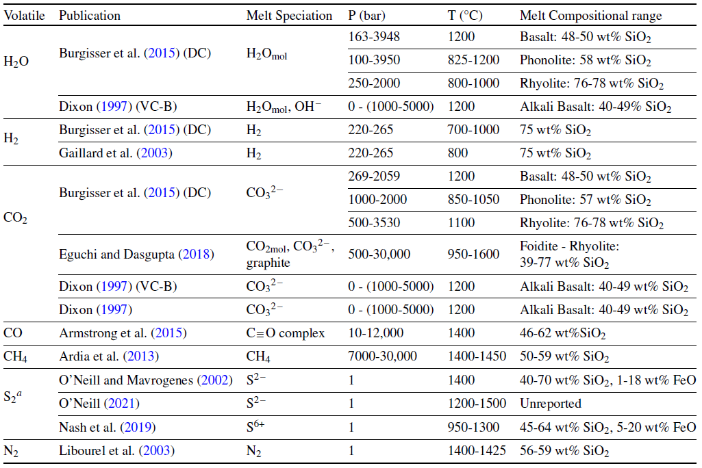
The solubility of a species is usually defined as the maximum concentration of a volatile which can remain in solution while co-existing with a pure gas phase of the same species. In a multicomponent system like that of EVo, it is assumed that the solubility of a species is related to the partial pressure/fugacity of the individual species \(i\). Over the past 30 years a plethora of solubility laws, particularly for H2O and CO2, have been developed. Different models for single species, or occasionally mixed H2O-CO2 volatiles are still being frequently introduced to the community; sometimes improvements based on new data, sometimes for a new P/T, \(f_{\ce{O2}}\), or silicate compositional regime. However, all these models are at least partially dependent on the abundance of the relevant species in the gas phase. In order to be as flexible as possible to different volcanic scenarios, and robust to future developments, EVo has been designed such that the user can select from a number of different solubility laws for various volatile species; it is also reasonably easy to add in additional solubility laws to a single file as they are released. In Table 1 below, the solubility laws for each species currently implemented in EVo are listed, along with the compositional, temperature, and pressure ranges they are calibrated for.
|
As is also discussed in Iacovino et al. (2021) and Wieser et al. (2022) with respect to the development of VESIcal (a Python3 engine for using and comparing a range of and solubility models), implementing the solubility laws which are published in academic papers is often problematic, particularly if the original work has not provided accompanying tools to benchmark against, given that some original manuscripts contain typos or formatting errors. Each of the solubility laws built into EVo are therefore provided in the API for the solubility_laws.py file, both for finding the abundance of a volatile in the melt based on gas phase fugacity, and for finding the reverse – the gas phase fugacity based on the concentration in the melt.
Both H and N form relatively simple binary volatile systems, present either in the gas phase, or dissolved in the silicate melt. However, C and S can both form additional phases: graphite in the case of carbon, and sulfide or anhydrite phases in the case of sulfur. In the case where graphite saturation occurs, CO2 solubility is forced to be calculated with Eguchi and Dasgupta (2018), which can account for both graphite and fluid saturation within the same equation. Sulfur solubility, and the way EVo handles both C and S saturation is covered in Handling additional phases: carbon and sulfur.
EVo takes into account the way that iron dissolved in the melt affects the redox state of the magma by modelling the exchange of oxygen, according to
This reaction is not calculated using an equilibrium constant, but the ratio of the molar fractions of and : \(F = X_{\ce{FeO}}/X_{\ce{Fe2O3}}\). This can be calculated using Kress and Carmichael (1991), or in the case of iron rich magma (total Fe \(>\)15 wt%) the model of Righter et al. (2013) which is calibrated for Martian melts. This exchange of oxygen between the silicate melt and the gas phase means that redox equilibrium is always maintained in the system.
Mass balance
As mentioned at the start of this section, the ‘mass balance and equilibrium constant’ method requires a set of mass balance equations along with the equilibrium constants already described. The total mass of each species in the magmatic system (\(W_{Ti}\)) is the sum its exsolved and dissolved components, thus
\(W_{gT}\) is the total weight fraction of gas in the system, \(w^v_i\) is the weight fraction of species i in the gas phase, and \(w^m_i\) is the weight fraction of species \(i\) in the melt. \(w^m_i\) is calculated according to a subset of the solubility laws listed in Table 1, and as such their dependencies differ according to the law and species in question; however, they are always dependent on the current pressure, and the fugacity of the corresponding species.
Mass conservation of volatile elements throughout the degassing process is enforced by keeping the total weight fraction of each element (\(W_{\mathrm{TH}}\), \(W_{\mathrm{TC}}\), \(W_{\mathrm{TO}}\), \(W_{\mathrm{TS}}\), \(W_{\mathrm{TN}}\)) constant
where \(W_Ti\) for each volatile species (not element) is calculated using (15), \(M_i\) is the molecular mass of species \(i\), \(W_{O(Fe)}\) is the weight fraction of oxygen held in iron (FeO/Fe2O3) within the melt, and \(W_{C(graph)}\) is the mass of graphite in the system (see Example of solving equations for the COHSN system).
In order to solve for the state of the magmatic system at a given temperature and pressure, equations for chemical equilibrium (1) to (5) and (14), solubility laws (Table 1) and mass conservation (10) and (16) to (20) are used jointly to algebraically reduce the system down to the smallest number of equations. In the case of the COHSN system, this is 4, which requires four variables to be solved for (\(X_{CO}\), \(X_{\ce{S2}}\), \(X_{\ce{O2}}\) and \(X_{\ce{N2}}\)). An example of how these equations are derived and then solved is shown for the COHSN system in Example of solving equations for the COHSN system. It is the case that the number of equations, and therefore variables, is always \(n-1\) for \(n\) number of volatile elements involved. These reduced equations are solved simultaneously, using an iterative method from the SciPy python package (Virtanen et al., 2020), conserving the mass fraction of each volatile element to a precision of 1 × 10⁻⁵.
Once a solution has been found for the speciation of the system at a single pressure, the volume of the gas phase (\(v\)) is calculated using
\(R\) is the universal gas constant (8.3144 J/mol K), \(\rho_l\) is the volatile-free melt density, calculated according to Lesher and Spera (2015), and \(\mu\) is the mean molecular weight of the gas phase, calculated as
Example of solving equations for the COHSN system
This section shows a worked example of how the full system of equations is algebraically reduced down to the four equations iterated to solve the system. In the COHSN system, the gas phase is made up of 10 species, in equilibrium at all times according to
where \(f_i\) is calculated according to (9). The variables to solve for are \(X_{CO}\), \(X_{\ce{S2}}\), \(X_{\ce{O2}}\) and \(X_{\ce{N2}}\), so the first aim is to calculate the mole fractions of all other species in terms of these 4 variables (written in blue, with derived species in red):
Note that \(X_{\ce{H2O}}\) is calculated by rearranging equations for \(K_1\), \(K_3\) and \(K_4\) in terms of \(f_{\ce{H2}}\), \(f_{\ce{CH4}}\) and \(f_{\ce{H2S}}\) respectively, and substituting these equations into (10) such that
This is re-arranged into quadratic form for \(X_{\ce{H2O}}\), and solved using the quadratic formula.
At this point, all 10 species in the gas phase can be described in terms of the 4 variables being solved for. As decompression occurs, mass conservation requires that the total amounts of each volatile element (COHSN) in the system remains constant. These mass conservation equations are set out in (16) to (20). In order to use the molar fractions derived above in (15), to replace the total amounts of each species \(W_{Ti}\) in (16) to (20), the molar fraction must be converted to weight fractions using
and the mass of the volatile dissolved in the melt must be calculated. Substituting (23) and solubility laws into (15) gives
where \(w^m_i(\dots)\) denotes the solubility law for species \(i\), which is dependent on \(X_i\), the pressure and temperature of the system, and in some cases other variables such as the \(f_{\ce{O2}}\) or silicate melt chemistry. \(w^m_i(\dots)\) returns the weight fraction of the species in the melt. As the gas weight fraction \(W_{gT}\) is the final unknown in the system, one of the mass conservation equations from eqs. (16) to (20) is re-arranged in terms of \(W_{gT}/\sum^{}_{j} X_jM_j\), thereby reducing the number of equations to solve down to 4. In the COHSN system, the conservation equation for nitrogen ((20)) is chosen, re-arranged to be substituted into the remaining conservation equations as
The system of 4 equations to be solved simultaneously can now be derived:
where \(melt\) is the major element composition of the silicate melt, and \(W_{O(Fe)}\) is the weight fraction of oxygen tied up in FeO and Fe2O3 within the silicate melt. This is controlled by the \(f_{\ce{O2}}\) of the system, and is calculated by finding \(F\), the ratio of FeO/Fe2O3 in the melt, using either Kress and Carmichael (1991) or Righter et al. (2013), then
These four equations are solved numerically using the SciPy optimize.fsolve function, formulated as a vector equality
The fsolve function makes an initial guess of the value for the vector \(\begin{bmatrix}X_{\ce{O2}}\\X_{\ce{CO}}\\X_{\ce{S2}}\\X_{\ce{N2}} \end{bmatrix}\), and then iterates, refining the guesses as appropriate until a solution is found. As the pressure is decreased in steps by EVo, the initial guess for each new pressure is the solution to the previous step. For the starting pressure, the entire system is constrained, so iteration is not required (see Run types, set-up options and input parameters for details on how this is achieved).
Handling additional phases: carbon and sulfur
The base degassing model described above deals with the case where there are 2 phases present: the silicate melt, containing a fraction of dissolved volatiles; and an exsolved gas phase. However, in the case of both C and S, additional phases can form outside of this 2-phase system. Here I describe how EVo handles these scenarios.
Carbon
A carbon-bearing system can become graphite saturated at low \(f_{\ce{O2}}\) (or, alternatively, diamond saturated at very high pressures; Holloway et al., 1992; LaTourrette and Holloway, 1994; Frost and Wood, 1997). Fig. 2 shows a simplified C-O magmatic system, illustrating the relationship between graphite and other phases. Note that EVo includes H which also interacts with C as CH4; however this has been excluded from Fig. 2 to clarify the relationship between graphite and the melt/volatile phase. At highly reduced conditions C may also be soluble in the silicate melt as a range of O and H-bearing species; however, as the species and reactions involved are still highly debated these have also been left off Fig. 2.
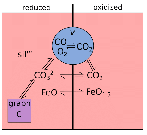
Fig. 2 A simple diagram of the C-O system in silicate melts. Each colour represents a different phase (gas/volatile (v), silicate melt (m) and a precipitated graphite phase). Phases and species which dominate under reducing conditions are to the left, while those which dominate under oxidising conditions are to the right. Two-way arrows indicate species that can interact within, and between different, phases.
In a graphite-saturated melt, the \(f_{\ce{CO2}}\) of the system is controlled by
As graphite is a pure, solid phase, it has a chemical activity of 1. The equilibrium constant equation for eq. (34) is therefore written as
showing that in a graphite saturated melt, \(f_{\ce{CO2}}\) is entirely controlled by the of the melt (Holloway et al., 1992). \(K_C\) is calculated according to the equation of Holloway et al. (1992),
with T in Kelvin and P in bar.
The silicate system in EVo is checked for graphite saturation by comparing the value of \(f_{\ce{CO2}}\) as calculated using the main model as described above (which assumes no graphite saturation), to that calculated using (35) (\(f_{\ce{CO2}, graphite}\)). If \(f_{\ce{CO2}, graphite} < f_{\ce{CO2}}\), then the melt must be graphite saturated (e.g., see Fig 7b of Eguchi and Dasgupta, 2018). If graphite saturation is found, EVo then forces the use of the Eguchi and Dasgupta (2018) model for CO2 solubility. The thermodynamics and structure of this model mean that it is applicable under both graphite and fluid saturated conditions, unlike the other option implemented in EVo, and can therefore be fed either \(f_{\ce{CO2}, graphite}\) or \(f_{\ce{CO2}}\).
Graphite saturation is only implemented in the ‘closed system’ degassing option; because in a closed system material cannot be removed, any graphite present in the melt at volatile saturation is assumed to decompress with the rest of the gas-melt system. The separate graphite phase decompresses with the gas-melt system, gradually depleting as carbon is degassed into the gas phase and the graphite phase replenishes the carbon dissolved in the melt (see Fig. 2). Graphite exhaustion (where the melt becomes graphite under-saturated) is detected if, to solve for a graphite saturated system, the graphite mass in the system must be negative. The system is first checked for graphite saturation during the setup of the system, and then after every pressure step if the system is not known to already be graphite-saturated.
When solving for a graphite-saturated system, the fugacity of all 3 carbon-bearing species can be determined solely using the \(f_{\ce{O2}}\) and (35). This removes an extra unknown from all systems containing carbon; in the example shown in Example of solving equations for the COHSN system, (29) is no longer used, and \(X_{\ce{CO}}\) is no longer a variable being solved for. The mass of the carbon reservoir is calculated as the difference between the total mass of carbon in the system and the mass calculated as being present in the gas and dissolved in the silicate melt.
Sulfur
As with carbon, the sulfur system has added complexities in that additional phases can form alongside the two accounted for in EVo (the silicate melt and gas phase). However, unlike with graphite saturation, there are two additional phases which have to be considered, the abundances of which vary according to \(f_{\ce{O2}}\). The simplified system is shown in Fig. 3, which similarly to Fig. 2 shows an idealised S-O system, excluding H.
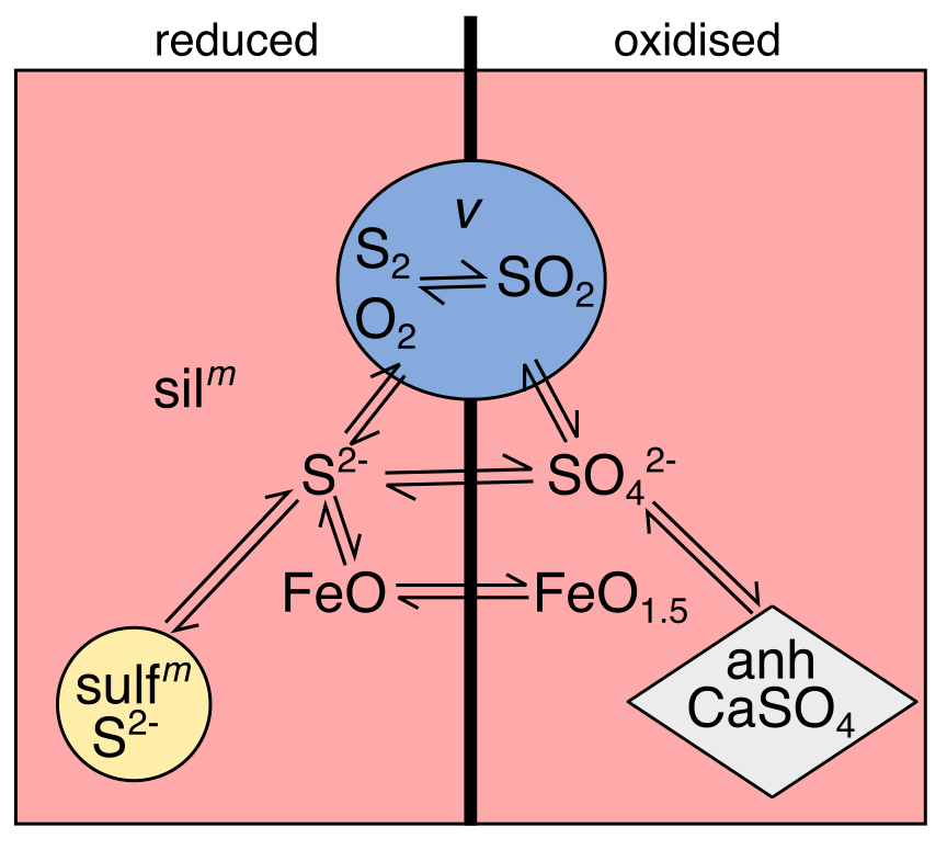
Fig. 3 A simple diagram of the S-O system in silicate melts. Each colour represents a different phase. Phases and species which dominate under reducing conditions are to the left, while those which dominate under oxidising conditions are to the right. Two-way arrows indicate species that can interact within, and between different, phases. Taken from Hughes et al. (2021).
Fig. 4 Sulfur speciation as a function of oxygen fugacity, after Jugo et al. (2010).
Under reducing conditions (approximately \(<\)FMQ, see Fig. 4) sulfur dissolves in silicate melts as S2-:
By comparison, under oxidised conditions, sulfur dissolves in the melt as SO42- through
where sulfur is instead in it’s S6+ state (Paris et al., 2001). It is well established from experimental studies that a silicate melt can contain S dissolved as one, the other, or both S2- and S6+ across the \(f_{\ce{O2}}\) range of terrestrial magmas (Carroll and Rutherford, 1988; Nilsson and Peach, 1993; Metrich and Clocchiatti, 1996). Magma produced on other planets across the solar system is thought to have an \(f_{\ce{O2}}\) which is less than the \(f_{\ce{O2}}\) of terrestrial mid-ocean ridge basalts (MORB, e.g., Schmidt et al., 2013b; Zolotov et al., 2013), which is well within the S2- stability field and is therefore expected to contain minimal S6+.
When a magma becomes sulfur-saturated, the phase precipitated is \(f_{\ce{O2}}\) dependent. A melt can become sulfide (S2-) saturated
or sulfate (SO42-) saturated (usually speciated as anhydrite, CaSO4). Silicate melts can also be multiply saturated with sulfide + sulfate \(\pm\) gas, resulting in a sulfur solubility maximum (Jugo, 2009; Hughes et al., 2021), with a corresponding solubility minimum where both S2- and S6+ are dissolved in approximately equal concentrations (Hughes et al., 2021). Due to the complexity of the sulfur system and the fact that the additional sulfide/sulfate phases are not pure S (as is the case for graphite), EVo follows the convention of other multi-component degassing models by not simulating magmas which are sulfur-saturated, in either phase (e.g., CHOSETTO, D-Compress: Moretti et al., 2003; Burgisser et al., 2015). Instead, EVo only deals with sulfur in the gas phase (speciated as S2, SO2 or H2S), and dissolved in the melt as either S2- or S6+.
The dissolution of S2 into a silicate melt has been shown experimentally to follow eq. (37) (O’Neill and Mavrogenes, 2002; O’Neill, 2021). As the \(\ce{O}^{2-}_{\mathrm{(melt)}}\) is viewed as a ‘structural element’ with abundances far greater than that of S2-, eq. (37) can define the solubility law for S2 as
where \(C_{\ce{S^{2-}}}\) is the ‘sulfide capacity’ of the melt (Fincham et al., 1954), analogous to the equilibrium constant \(K\) of (37). \(C_{\ce{S^{2-}}}\) is highly compositionally dependent and can, for given pressure and temperature conditions, be reformulated as a constant for a given melt composition. Those parametrisations for \(C_{\ce{S^{2-}}}\) which are implemented as options in EVo are listed in Table 1. While (38) can similarly be re-arranged to generate a sulfate capacity \(C_{\ce{S^{6+}}}\) (Fincham et al., 1954)
at the time of writing no experimental validation (on magmatically relevant silicate compositions), nor expressions equivalent to those provided by, e.g., O’Neill (2021) for \(C_{\ce{S^{2-}}}\) have been published – although results mentioned in abstract (O’Neill and Mavrogenes, 2019) confirm the relationship and suggest an expression for \(C_{\ce{S^{6+}}}\) may be forthcoming. To determine the amount of in the melt, EVo instead uses Nash et al. (2019) which calculates the ratio of S6+/S2- as
for temperatures (T) of 1000 - 2000 K.
The amount of S2- which can be dissolved in a silicate melt at sulfide saturation, controlled by (39), is referred to as the “Sulfide Content at Sulfide Saturation”, or SCSS. The SCSS has been extensively studied over the past few decades (O’Neill and Mavrogenes, 2002; Liu et al., 2007; Fortin et al., 2015; Wykes et al., 2015; Smythe et al., 2017; O’Neill, 2021), and in EVo is calculated using the model of Liu et al. (2007). EVo checks for sulfide saturation by comparing \(w^m_{\ce{S^{2-}}}\) as calculated using (40) to the SCSS. If \(w^m_{\ce{S^{2-}}}\) \(\geq\) SCSS, then the melt is sulfide saturated and EVo produces a warning stating that sulfide saturation has been reached, and the model is no longer valid.
Run types, set-up options and input parameters
Two different run types can be performed while calculating a decompression path: “Closed system” or “Open system”. Closed-system runs, the default, assume that the gas is in equilibrium with the melt and there is no physical-chemical separation between the two phases. This models a system where the gas bubbles are entrained in the melt and rise at the same speed as the magma.
In open-system degassing, a fraction of the gas released as a magma decompresses is assumed to be lost (or chemically isolated) from the melt as it is produced, mimicking a scenario where gas bubbles rise to the surface through a magma. EVo simulates this by resetting the gas fraction after every pressure step
where \(dP\) is the pressure step (bar) and \(a\) is the fraction of the gas phase which is removed from the system after each increment (using \(a\) rather than fully removing all exsolved volatiles allows for an exploration of efficient vs inefficient open-system degassing). Once \(W_{gT}\) has been reset, the new masses of the volatile elements left in the system are calculated before the pressure is incremented. EVo tracks the evolution of the magma as a function of pressure in this scenario, and does not track the accumulated composition of the degassed volatiles, although it does provide the chemistry of the instantaneous exsolved gas phase at each pressure step.
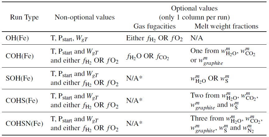
There are three different options which can be used to set-up EVo for a decompression calculation, discussed below. These options can also be used to find the equilibrium conditions at a single pressure, either at a set pressure using option (1), or the volatile saturation pressure, found using either (2) or (3).
1) Where \(P_{start}\) and \(W_{gT}\) are known
Where the gas mass fraction is known at the pressure of interest (either for the start of a degassing run or to calculate the composition at a single point), along with the temperature, the state of the system can be found using a subset of additional parameters as described in Table 2.
|
Using these input values, all other relevant parameters for the initial conditions can be calculated. Where a melt weight fraction of a volatile is provided, the respective fugacity is calculated using the solubility laws.
Solubility models usually provide analytical expressions for the concentration of a volatile species dissolved in a magma as a function of either partial pressure, or fugacity. Analytical expression for the inverse (calculating the fugacity of a species given the concentration dissolved in the melt) are usually not provided, and in some cases cannot be found by simple re-arrangement; in these cases (both the models of Dixon (1997) and Eguchi and Dasgupta (2018)) numerical methods are used to obtain the correct fugacity.
The 1-4 fugacities (depending on the number of elements considered), P, T, reactions Eqs. (1) to (5) and (10) are then used algebraically to find all \(X_i\) and \(f_i\). Once all molar fractions have been calculated, the masses of each element in the system can be computed (Eqs. (16) to (20)), along with the mass of oxygen fixed by FeO* using (30).
2) Calculating \(P_{sat}\), the volatile saturation pressure
In many scenarios, having to specify a starting pressure and gas fraction in order to model a decompression path is inconvenient, as these variables are often unknown. Instead, it is preferable to calculate the saturation pressure for a given system volatile content (e.g., the H2O and CO2 concentration of the melt prior to the onset of degassing), and start the decompression from there. EVo allows this setup option by asking for the \(f_{\ce{O2}}\) at the point of volatile saturation (usually taken to be the \(f_{\ce{O2}}\) of the magma source), and the undegassed volatile content of the melt.
When the saturation pressure of a magma with a given dissolved volatile concentration is found, the following equality holds:
where \(P\) is the total pressure and \(P_i\) is the partial pressure of species \(i\) calculated according to it’s corresponding solubility law, for a fixed concentration in the melt. The saturation pressure is found by numerically solving (44) for \(P\), where
using the Brent method as implemented in SciPy (Virtanen et al., 2020). This method was chosen as it allows the solution to be bracketed; this prevents the numerical solver guessing a negative pressure which is invalid within the inverted solubility laws. Once \(P_{sat}\) has been found, \(W_{gT}\) is set to 1×10⁻⁶ wt% (an arbitrarily small number sufficiently close to zero to not affect the results but successfully initialise the calculation), the atomic volatile masses in the system are calculated as in eqs. (16) to (20) and decompression steps can commence.
3) Calculating \(P_{sat}\) and volatile speciation
The above two setup options work well for use-cases such as modelling the degassing path of volcanic samples, or single volcanic systems where the starting conditions (e.g., \(f_{\ce{O2}}\), volatile content) are similar. However, in planetary science a key component of research is comparing the gas phase/atmospheres produced when the only variable is the starting \(f_{\ce{O2}}\). In set-up options 1 & 2, this poses a problem when dealing with volatile elements which exist as multiple dissolved species, particularly for H and C.
Using the simple case of the H2O-O2-H2 system, H in the melt can be dissolved either as H2O, or H2, although in oxidised to moderately reduced magmas, as seen on Earth, the H2 component is minimal. A fixed magmatic H2O content imposes a constant \(f_{\ce{H2O}}\); since the is being lowered, \(f_{\ce{H2}}\) must increase to maintain equilibrium. A greater \(f_{\ce{H2}}\) also enforces a higher magma content; therefore, as the \(f_{\ce{O2}}\) of a magma is decreased with a fixed H2O content, the dissolved H2 must increase proportionally (Fig. 5).
Fig. 5 The mass of H2O, H2 and total H in the silicate melt at volatile saturation, when the enforced saturation conditions are \(f_{\ce{O2}}\) and the dissolved H2O content.
When comparing degassing regimes where the \(f_{\ce{O2}}\) is varied, Fig. 5 shows it is not sufficient to simply fix the magma volatile content using a single species. E.g., volcanic gases released at FMQ compared to FMQ-6 in Fig. 5 cannot be directly compared, as the more reduced scenario has almost double the amount of H dissolved in the melt at the point of volatile saturation, hence the \(f_{\ce{O2}}\) is not the only factor being varied. Instead, for meaningful isolation of the effects of \(f_{\ce{O2}}\) changes alone, the total mass of each volatile element must be enforced, with the speciation at volatile saturation allowed to vary freely according to the \(f_{\ce{O2}}\) conditions.
Similarly to set-up option 2, this is solved numerically. EVo is initialised with the \(f_{\ce{O2}}\) at volatile saturation, and the total atomic masses of each volatile element in the system. The solver then guesses the proportion of each element which is dissolved as H2O, CO2, S2- and N2, with the remainder dissolved as other species, or in the gas phase (which is minimal at volatile saturation, but relevant in order for the system of equations to work). As in the main model, a system of 4 equations (for the COHSN system) is solved simultaneously:
This is similar in form to eq. (31), but in this case the variables are the mass fractions of dissolved volatiles, rather than the molar fractions of species in the gas phase. When a guess is made for (46) (structured as the vector \(\begin{bmatrix}w^m_{\ce{|H2O|}}\\w^m_{\ce{CO2}}\\w^m_{\ce{S^{2-}}}\\w^m_{\ce{N2}}\end{bmatrix}\)), it is first passed to (44) to find the saturation pressure, \(P_{sat}\), before the \([W_i]_{predicted}\) values are calculated. The key difference between this setup option and options 1 & 2 is that in this case the mass of each element in the system is known and the speciation is calculated; in the previous cases a subset of the melt or gas phase speciation is known and the solution finds the total masses of each element.
Benchmarking
During the development of EVo, individual elements of the model were each tested to ensure correct implementation. For example, the Kress and Carmichael (1991) relationship between \(f_{\ce{O2}}\) and ferric/ferrous iron was tested against the spreadsheet of Iacovino (2021), and individual solubility laws were tested either against the relevant published calculator (e.g., excel spreadsheets in the case of Newman and Lowenstern, 2002; Eguchi and Dasgupta, 2018), or against figures in the original publication where these were not provided.
EVo has also been initially tested against DCompress to ensure numerical accuracy in the thermodynamic calculation of the gas phase chemistry. In order to maximise similarity between the two models, for this comparison EVo is run using the H2O, H2 and CO2 solubility laws implemented by Burgisser et al. (2015) in DCompress; to distinguish this setup from EVo under standard run conditions (with H2 and CO2 solubility laws from Gaillard et al. (2003) and Eguchi and Dasgupta (2018), respectively), this version is referred to as EVo(DC). The two major differences left between the two models are therefore the treatment of sulfur solubility (EVo uses the sulfide capacity, as described in Handling additional phases: carbon and sulfur, while DCompress has a solubility law for SO2 and H2S), and the source of the equilibrium constants. DCompress uses equations from Ohmoto and Kerrick (1977) to calculate equilibrium constants K1-K5, while EVo and EVo(DC) calculate them using more recent thermochemical data from Chase (1998) as described in Overview of the chemical model. The differences between the two methods in K1-5 are shown in Fig. 6.
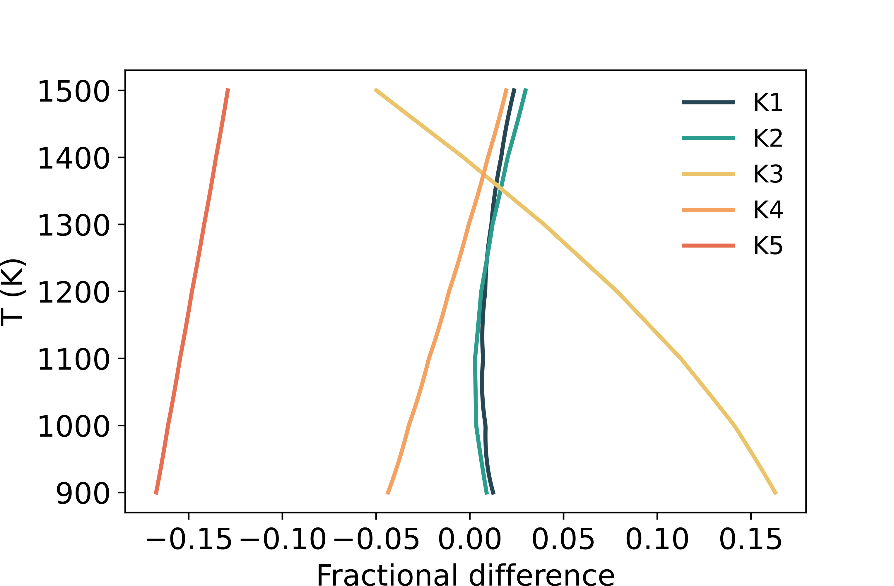
Fig. 6 The difference between the equilibrium constants as calculated in DCompress and EVo, expressed as K1(EVo)/K1(DC).
EVo(DC) and DCompress were run at a single pressure, using input method (1) as described in 1) Where P_{start} and W_{gT} are known, a gas weight fraction of 0.001%, and other parameters as listed on the individual panels within Fig. 7 to compare the calculation of the gas phase chemistry.
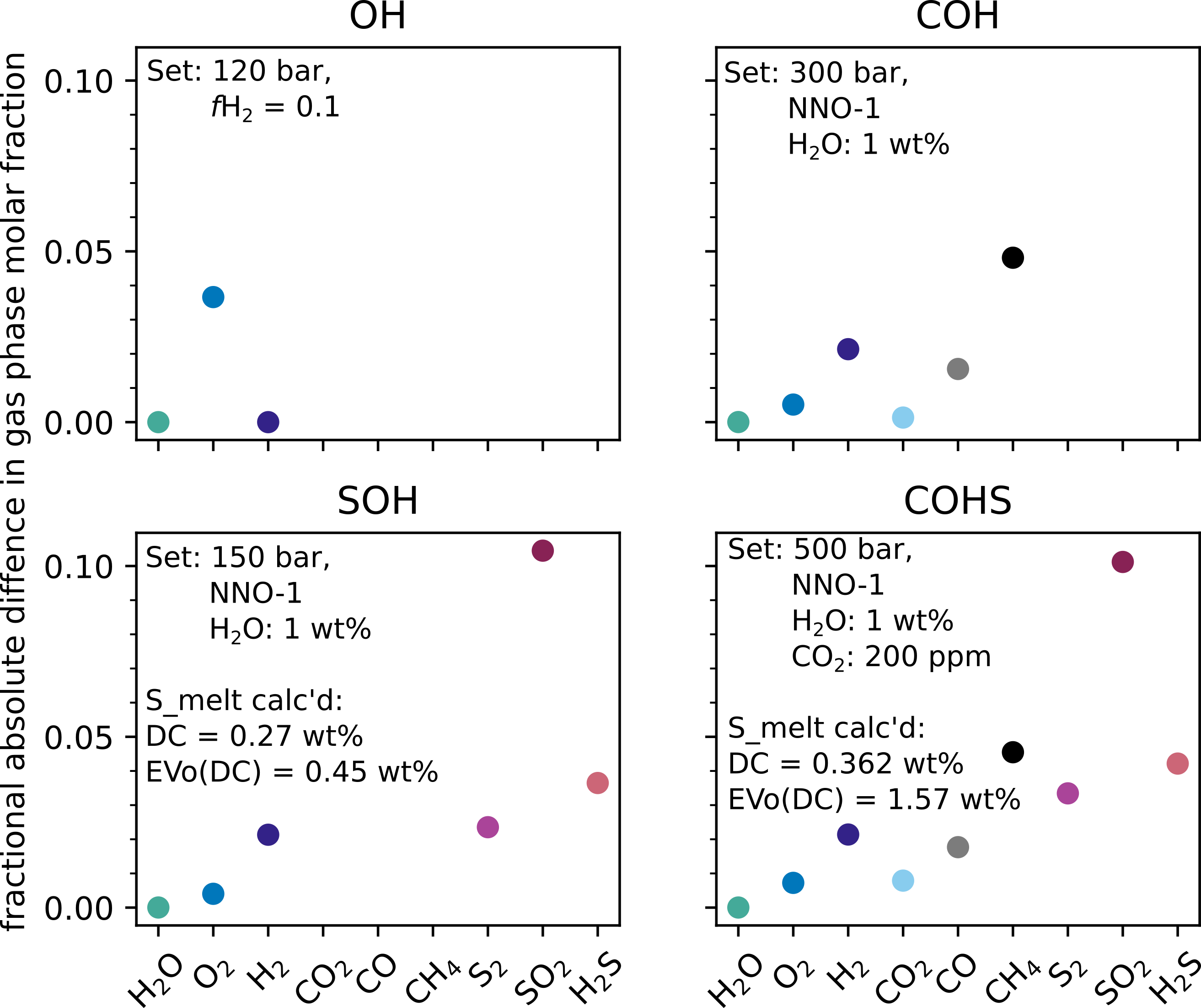
Fig. 7 The absolute fractional difference (calculated as \(\lvert X_{i, \mathrm{EVo(DC)}} - X_{i, \mathrm{DC}} \rvert/X_{i, \mathrm{DC}}\) where \(X_i\) is the mole fraction of each species \(i\)) between the gas phase speciation of DCompress and EVo(DC) when setup with the same input parameters. The magma composition used in the calculations is the default basalt composition for DCompress
In the case of the OH and COH systems, the difference between the results of the two models are \(\leq\) 5% for each species. These differences can be largely explained by differences in the value of equilibrium constants K1, K2 and K3 (Fig. 6). These differences in the OH/C systems can be reduced to \(\leq\) 1% by using the equilibrium constants from DCompress in EVo(DC). The particularly large difference on K5 at 1473 K is responsible for the largest difference between the two models, in the SOH and COHS setups. As the gas phase speciation is determined first using this method, and the melt S content is calculated based on the gas fugacity, the sulfur solubility law does not affect the gas phase speciation in this example; however the difference in the amount of sulfur dissolved in the melt is shown in the SOH and COHS panels of Fig. 7, as calculated by the different solubility laws.
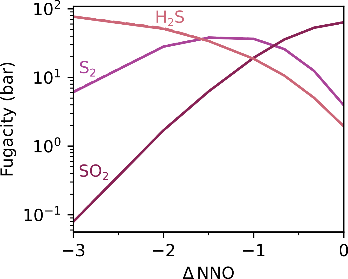
Fig. 8 Gas phase fugacities for the sulfur species. Both EVo and DC have been plotted, differences are within the linewidth.
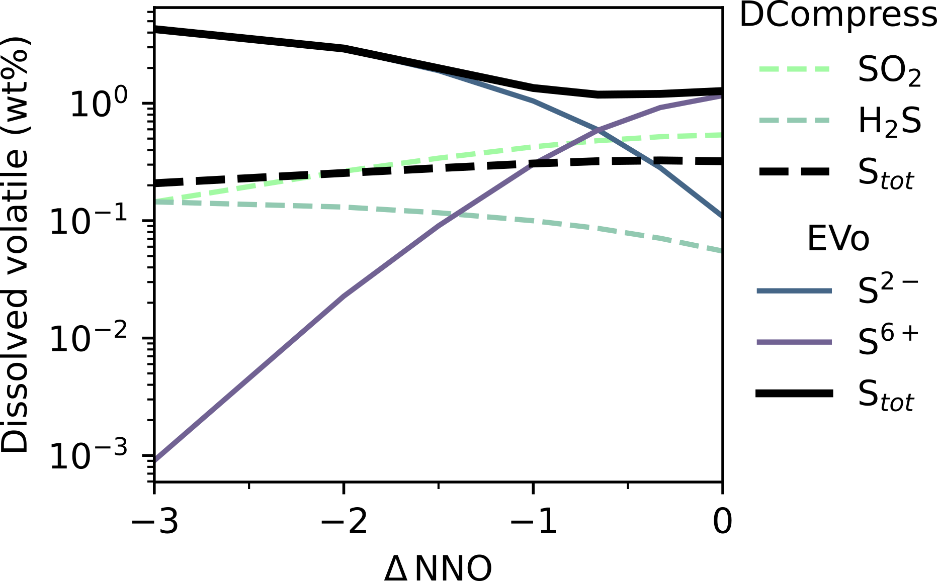
Fig. 9 Dissolved sulfur species
The difference in the treatment of sulfur solubility between DCompress and EVo is demonstrated in Fig. 8 and Fig. 9. When given the same gas-phase fugacities for S2, SO2 and H2S across an \(f_{\ce{O2}}\) range, EVo consistently predicts a higher total dissolved S content, following an experimentally well-established trend that in reduced melts (where sulfur dissolves as S2- ), the solubility of sulfur increases with reducing \(f_{\ce{O2}}\) (e.g., Fincham et al., 1954; Katsura and Nagashima, 1974; Backnaes and Deubener, 2011; Lesne et al., 2015). In contrast, DCompress predicts a largely constant total sulfur content, decreasing slightly with reducing \(f_{\ce{O2}}\).
Decompression benchmarking
I now compare the results of EVo (now using it’s default solubility laws) to those of 3 different models of volcanic degassing which include sulfur: DCompress (Burgisser et al., 2015), SolEx (Witham et al., 2012) and Chosetto, the newly released implementation of Moretti et al. (2003). Two decompression runs are shown in Fig. 10, one oxidised with an of NNO+0.5, and one slightly reduced at NNO-2. SolEx is only shown in the oxidised example, as it cannot be run with an lower than NNO+0.5. All 4 models were initialised with 1 wt% , 500 ppm and 3000 ppm S. Only EVo has the option to automatically find the volatile saturation point; SolEx begins all runs at 4000 bar, while DCompress was run by adjusting the starting pressure until the total sulfur content matched the required 3000 ppm and Chosetto’s starting pressure was adjusted until it could numerically resolve.
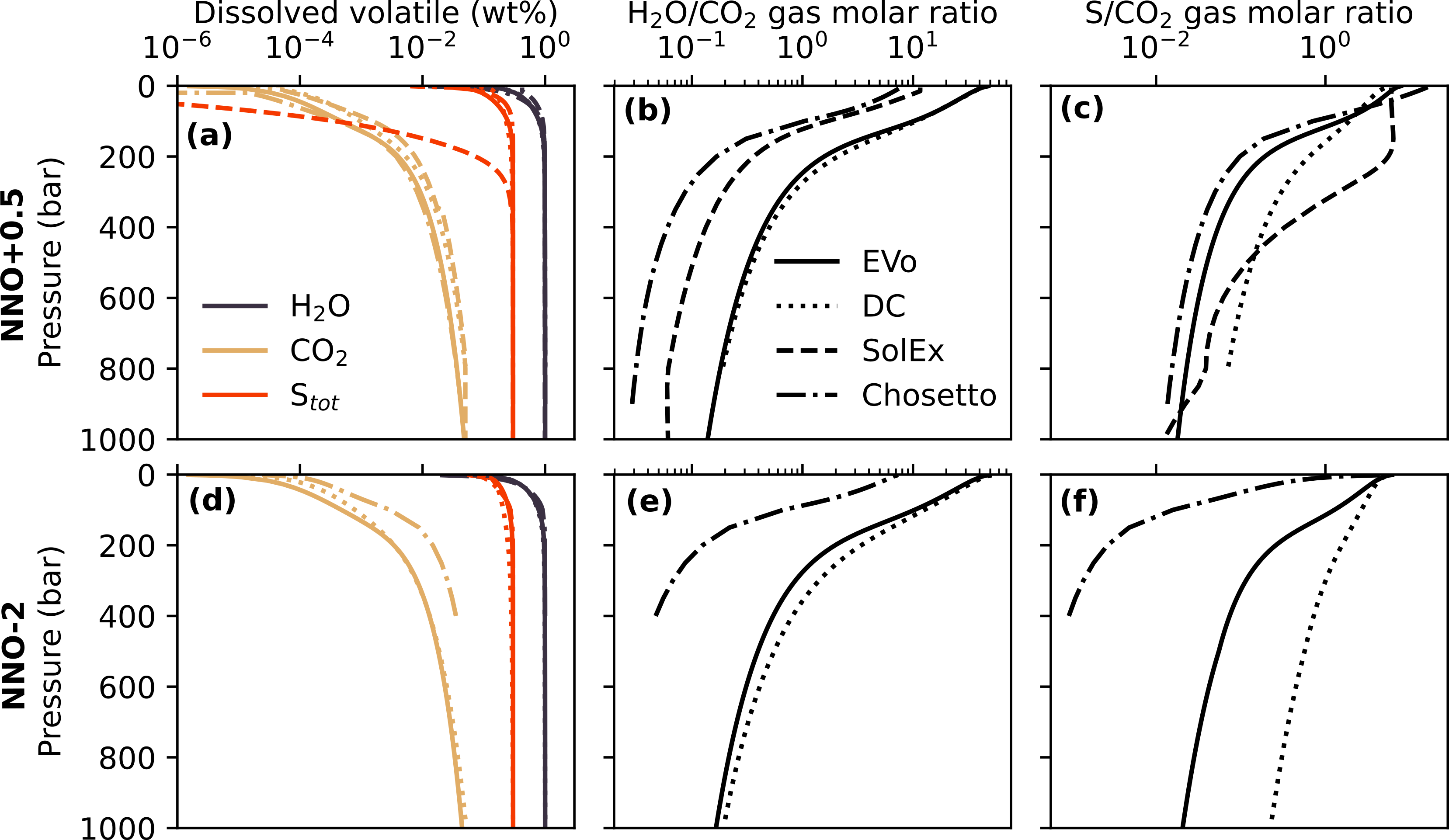
Fig. 10 The melt volatile content, H2O/CO2 ratio and S/CO2 ratio in the gas phase for 4 different models during decompression. Each model was initiated with 1 wt%H2O, 500 ppm CO2 and 3000 ppm S. EVo is the only model which allows the saturation pressure to be found automatically; SolEx always starts at 4000 bar, Psat was found manually for DCompress and Chosetto. At NNO-2, Chosetto was started at the first point it could numerically resolve.
Fig. 10 shows (a) the volatile content of the melt, (b) the H2O/CO2 ratio in the gas phase and (c) the S/CO2 ratio of the gas phase. All 4 models show close agreement on the dissolved volatile content as the pressure decreases, aside from the SolEx S content, which starts to rapidly decrease at a much higher pressure than other models in Fig. 10 a. Chosetto also shows a higher content in the melt in Fig. 10 d. All 4 models also show similar trends in the H2O/CO2 ratio, although both SolEx and Chosetto both have systematically more CO2-rich gases.
The largest difference between models lies in the behaviour of sulfur during degassing. SolEx shows sulfur degassing at much higher pressures than other models, while DCompress produces a more gradual release with pressure. EVo most closely resembles Chosetto under oxidised conditions, with sulfur starting to rapidly degas at 200 bar. Under reduced conditions the differences between models grow greater; the difference between Chosetto and EVo potentially being due to the presence of CO and CH4 in the gas phase of EVo while Chosetto only considers CO2.
The benchmarking comparisons shown in this section indicate that EVo compares well to other publish models for multi-species volcanic degassing. Where models differ, for example in the COHS subplot of Fig. 7, the driving factors are well understood. The lack of a standard method/dataset with which to benchmark and compare such models, which often only show subsets of the common volatile species or differ in other substantive ways, is an issue across Earth Sciences; however, Fig. 10 shows that on a limited dataset, EVo follows similar trends to all three of the other published models which include sulfur in their parametrisations, with the exception of the sulfur/ behaviour in SolEx, which appears to be an outlier.